


See through your quantum program: Classiq’s new QP visualization trick


Ever tried to debug a quantum circuit and lost track of which qubits are controlling which operations? Same here — until I tried Classiq’s updated Quantum Program (QP) Visualization.
A recent release added a subtle but game-changing improvement: controlled functions are displayed as transparent blocks, while target variables remain filled.
This simple visual cue makes it obvious which quantum variables are acting as controls and which operations are being applied — whether that’s to a single qubit or a high-level QMOD variable.
⚙️ How it works
- Transparent “control” blocks – The empty outline shows where a function is conditionally applied. You can see the control line or variable passing through it.
- Filled target blocks – The opaque sections highlight the operations acting on target variables.
- Visual clarity – By separating control from target, the circuit becomes easier to read and debug — especially for nested control structures and variable hierarchies.
🧩 Examples
🖼 Example 1 – Single-variable control
qfunc main(output target: qbit) {
qb: qbit;
allocate(qb);
H(qb);
allocate(target);
control (qb) {
X(target);
}
}
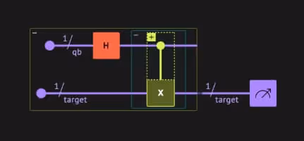
Here, a single quantum variable qb controls an X operation on target.
The outlined block around qb highlights its role as the controller, while the filled X shows the action on the target.
View this quantum program visualization in Classiq Platform
🖼 Example 2 – Multi-qubit control
qfunc my_mcx(cntrl: qbit[], target: qbit) {
control (cntrl) {
X(target);
}
}
qfunc main(output cntrl: qbit[], output target: qbit) {
allocate(50, cntrl);
allocate(target);
my_mcx(cntrl, target);
}
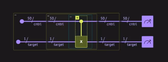
This example shows a multi-qubit control scenario. The transparent block spans the array cntrl, while the filled X gate acts on the target variable target. The visualization makes it effortless to see both the structure and the scale of the control.
View this quantum program visualization in Classiq Platform
🖼 Example 3 – Nested control & parameterized power
qfunc main(output x: qbit, output ctrl: qbit[]) {
allocate(2, ctrl);
hadamard_transform(ctrl);
allocate(x);
control (ctrl) {
power (3) {
H(x);
}
}
}
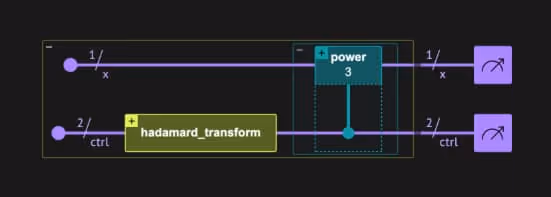
In this nested example, the control array ctrl governs a parameterized power operation, which applies a Hadamard transform on x. The transparent control region around the power(3) block makes the control flow obvious even in deeper hierarchies.
View this quantum program visualization in Classiq Platform
💡 Why it matters
- Faster debugging – No more guessing which function is conditional; the control/target relationship is visible at a glance.
- Readable and scalable – Works cleanly from small examples to complex QMOD programs with dozens of quantum variables.
- Better communication – Makes it easier to discuss program structure with both technical and non-technical audiences.
🧑💻 Ready to try?
If you’re already using Classiq Studio or the Python SDK, you’ll see this improvement automatically the next time you visualize a program. New users can explore it at classiq.io and see how easy it is to design, debug, and share quantum programs.
Ever tried to debug a quantum circuit and lost track of which qubits are controlling which operations? Same here — until I tried Classiq’s updated Quantum Program (QP) Visualization.
A recent release added a subtle but game-changing improvement: controlled functions are displayed as transparent blocks, while target variables remain filled.
This simple visual cue makes it obvious which quantum variables are acting as controls and which operations are being applied — whether that’s to a single qubit or a high-level QMOD variable.
⚙️ How it works
- Transparent “control” blocks – The empty outline shows where a function is conditionally applied. You can see the control line or variable passing through it.
- Filled target blocks – The opaque sections highlight the operations acting on target variables.
- Visual clarity – By separating control from target, the circuit becomes easier to read and debug — especially for nested control structures and variable hierarchies.
🧩 Examples
🖼 Example 1 – Single-variable control
qfunc main(output target: qbit) {
qb: qbit;
allocate(qb);
H(qb);
allocate(target);
control (qb) {
X(target);
}
}
Here, a single quantum variable qb controls an X operation on target.
The outlined block around qb highlights its role as the controller, while the filled X shows the action on the target.
View this quantum program visualization in Classiq Platform
🖼 Example 2 – Multi-qubit control
qfunc my_mcx(cntrl: qbit[], target: qbit) {
control (cntrl) {
X(target);
}
}
qfunc main(output cntrl: qbit[], output target: qbit) {
allocate(50, cntrl);
allocate(target);
my_mcx(cntrl, target);
}
This example shows a multi-qubit control scenario. The transparent block spans the array cntrl, while the filled X gate acts on the target variable target. The visualization makes it effortless to see both the structure and the scale of the control.
View this quantum program visualization in Classiq Platform
🖼 Example 3 – Nested control & parameterized power
qfunc main(output x: qbit, output ctrl: qbit[]) {
allocate(2, ctrl);
hadamard_transform(ctrl);
allocate(x);
control (ctrl) {
power (3) {
H(x);
}
}
}
In this nested example, the control array ctrl governs a parameterized power operation, which applies a Hadamard transform on x. The transparent control region around the power(3) block makes the control flow obvious even in deeper hierarchies.
View this quantum program visualization in Classiq Platform
💡 Why it matters
- Faster debugging – No more guessing which function is conditional; the control/target relationship is visible at a glance.
- Readable and scalable – Works cleanly from small examples to complex QMOD programs with dozens of quantum variables.
- Better communication – Makes it easier to discuss program structure with both technical and non-technical audiences.
🧑💻 Ready to try?
If you’re already using Classiq Studio or the Python SDK, you’ll see this improvement automatically the next time you visualize a program. New users can explore it at classiq.io and see how easy it is to design, debug, and share quantum programs.